Page 16 - MSDN Magazine, February 2018

Azure. Note that a new browser tab or window will open and that the interface looks more like the screen in Figure 1. Click inside the text box and write the following code:
print("Hello World!")
Choose Run Cells from the Cell menu at the top of the page. The screen should look like Figure 2.
Click inside the blank cell that
Jupyter added and choose Cell > Cell
Type > Markdown from the menu bar. Then add the following text.
# This is markdown text #
Markdown is a versatile and lightweight markup language.
Click the save icon and close the browser tab. Back in the Library window, click on the notebook file again. The page will reload and the markdown formatting will take effect.
Next, add another code cell, by clicking in the markdown cell and choosing Insert Cell Below from the Insert menu. Previously, I stated that only Python code could be executed in Python notebook. That is not entirely true, as you can use the “!” command to issue shell commands. Enter the following command into this new cell.
! ls -l
Choose Run Cells from the Run menu or click the icon with the Play/Pause symbol on it. The command returns a listing of the contents of the directory, which contains the notebook file and the README.md file. Once again, Jupyter added a blank cell after the response. Type the following code into the blank cell:
%matplotlib inline
import numpy as np
import matplotlib.pyplot as plt x = np.random.rand(100)
y = np.random.rand(100) plt.scatter(x, y)
plt.show()
Run the cell and after a moment a scatter plot will appear in the results. For those familiar with Python, the first line of code may look unfamiliar, as it is part of the IPython kernel which executes Python code in a Jupyter notebook.
Figure 2 Hello World! in a Jupyter Notebook
Python (matplotlib.org). The code then generates two arrays of 100 random numbers and plots the results as a scatter plot. The final line of code displays the graph. As the numbers are randomly gen- erated, the graph will change slightly each time the cell is executed.
Notebooks in ML Workbench
So far, I have demonstrated running Jupyter networks as part of the Azure Notebook service in the cloud. However, Jupyter note- books can be run locally, as well. In fact, Jupyter notebooks are integrated into the Azure Machine Learning Workbench product. In my previous article, I demonstrated the sample Iris Classification project. While the article did not mention it, there is a notebook included with the project that details all the steps needed to create a model, as well as a 3D plot of the iris dataset.
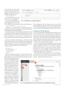
To view it, open the Iris Classifier sample project from last month’s column, “Creating Models in Azure ML Workbench” (msdn.com/ magazine/mt814992). If you did not create the project, follow the directions in the article to create a project from the template. Inside the project, shown in Figure 3, click on the third icon (1) from the top of the vertical toolbar on the left-hand side of the window, then click on iris (2) in the file list.
The notebook file loads, but the notebook server is not running— the results shown are cached from a previous execution. To make the notebook interactive, click on the Start Notebook Server (3) button to activate the local notebook server.
The command %matplotlib inline instructs the IPython runtime to display graphs generated by matplotlib in-line with the results. This type of command, known as a “magic” command, starts with “%”. A full exploration of magic com- mands warrants its own article. For further information on magic commands, refer to the IPython documentation at bit.ly/2CfiMvh.
For those not familiar with Python, the previous code segment imports two libraries, NumPy and Matplotlib. NumPy is a Python package for scientific computing (numpy.org) and Matplotlib is a pop- ular 2D graph plotting library for
12 msdn magazine
Figure 3 Viewing Notebooks in an Azure Machine Learning Workbench Project
Artificially Intelligent