Page 60 - MSDN Magazine, June 2017

The result of posGrad - negGrad is:
000 0 0 -1 0 +1 -1 0+1-1 000 000
If you review the algorithm carefully, you’ll see that cell values in the delta gradient matrix can only be one of three values: 0, +1 or -1. Delta gradient values of +1 correspond to weights that should be increased slightly. Values of -1 correspond to weights that should be decreased slightly. Clever! The amount of increase or decrease is set by a learn- ing rate value. So the weight from visible[1] to hidden[2] would be decreased by 0.01 and the weight from visible[2] to hidden[1] would be increased by 0.01. A small learning rate value makes training take longer, but a large learning rate can skip over good weight values.
Figure 3 Demo of a Restricted Boltzmann Machine 56 msdn magazine
So, how many iterations of training should be performed? In general, setting the number of training iterations and choosing a value of the learning rate are matters of trial and error. In the demo program that accompanies this article, I used a learning rate of 0.01 and a maximum number of iterations set to 1,000. After training, I got the weights and bias values shown in Figure 1.
Interpreting a Restricted Boltzmann Machine
OK, so it’s possible to take a set of data where each value is zero or one, then set a number of hidden nodes, and get some weights and bias values. What’s the point?
One way to think of an RBM is as a kind of compression machine. For the example film preference data, if you feed a type A person as input (1, 1, 0, 0, 0, 0), you’ll usually get (1, 1, 0) as output. If you feed (1, 1, 0) as input to the hidden nodes, you almost always get (1, 1, 0, 0, 0, 0) as output in the visible nodes. In other words, (1, 1, 0, 0, 0, 0) and slight variations are mapped to (1, 1, 0). This behavior is closely related to, but not quite the same as, factor analysis in classical statistics.
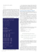
Take a look at the demo program in Figure 3. The demo cor- responds to the film like-dislike example. The demo creates a 6-3 RBM and trains it using the 12 data items presented in the previous section. The hardcoded data is set up like so:
int[][] trainData = new int[12][]; trainData[0] = new int[] { 1, 1, 0, 0, 0, 0 }; trainData[1] = new int[] { 0, 0, 1, 1, 0, 0 }; ...
trainData[11] = new int[] { 0, 0, 1, 0, 1, 1 };
In most situations you’d read data from a text file using a helper method. The demo RBM is created and trained like this:
int numVisible = 6;
int numHidden = 3;
Machine rbm = new Machine(numVisible, numHidden); double learnRate = 0.01;
int maxEpochs = 1000;
rbm.Train(trainData, learnRate, maxEpochs);
A small learning rate value makes training take longer, but a large learning rate can skip over good weight values.
The choice of setting the number of hidden nodes to three was arbitrary and the values for learnRate and maxEpochs were deter- mined by trial and error. After training, the RBM is exercised like this:
int[] visibles = new int[] { 1, 1, 0, 0, 0, 0 }; int[] computedHidden = rbm.HiddenFromVis(visibles); Console.Write("visible = ");
ShowVector(visibles, false);
Console.Write(" -> "); ShowVector(computedHidden, true);
If you experiment with the code, you’ll notice that the computed hidden values are almost always one of three patterns. Person type A (or weak or noisy version) almost always generates (1, 1, 0). Type B generates (1, 0, 1). And type C generates (0, 1, 1). And if you feed the three patterns as inputs, you’ll almost always get the three
Test Run