Page 58 - MSDN Magazine, June 2017

TesT Run JAMES MCCAFFREY Restricted Boltzmann Machines Using C#
A restricted Boltzmann machine (RBM) is a fascinating software component that has some similarities to a basic neural network. An RBM has two sets of nodes—visible and hidden. Each set of nodes can act as either inputs or outputs relative to the other set. Each node has a value of zero or one and these values are calculated using probability rather than deterministically.
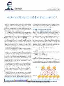
Each visible-layer node is conceptually connected to each hidden- layer node with a numeric constant called a weight, typically a value between -10.0 and +10.0. Each node has an associated numeric constant called a bias. The best way to start to understand what an RBM is is by way of a diagram. Take a look at Figure 1.
In Figure 1, the visible nodes are acting as the inputs. There are six visible (input) nodes and three hidden (output) nodes. The values of the visible nodes are (1, 1, 0, 0, 0, 0) and the computed values of the hidden nodes are (1, 1, 0). There are 6 * 3 = 18 weights connecting the nodes. Notice that there are no visible-to-visible or hidden-to-hidden weights. This restriction is why the word “restricted” is part of the RBM name.
Each of the red weight arrows in Figure 1 points in both direc- tions, indicating that information can flow in either direction. If nodes are zero-base indexed, then the weight from visible[0] to hidden[0] is 2.78, the weight from visible[5] to hidden[2] is 0.10 and so on. The bias values are the small green arrows pointing into each node so the bias for visible[0] is -0.62 and the bias for hidden[0] is +1.25 and so on. The p value inside each node is the probability that the node takes a value of one. So, hidden[0] has p = 0.995, which means that its calculated value will almost certainly be one, and in fact it is, but because RBMs are probabilistic, the value of hidden[0] could have been zero.
You probably have many questions right about now, such as where the weights and bias values come from, but bear with me—you’ll see how all the parts of the puzzle fit together shortly. In the sections that follow, I’ll describe the RBM input-output mechanism, explain where the weights and bias values come from, present a demo pro- gram that corresponds to Figure 1, and give an example of how RBMs can be used.
This article assumes you have intermediate or better program- ming skills, but doesn’t assume you know anything about RBMs. The demo program is coded using C#, but you should have no trouble refactoring the code to another language such as Python or JavaScript if you wish. The demo program is too long to present
in its entirety, but the complete source code is available in the file download that accompanies this article. All error checking was removed to keep the main ideas as clear as possible
The RBM Input-Output Mechanism
The RBM input-output mechanism is (somewhat surprisingly) relatively simple and is best explained by an example. Suppose, as in Figure 1, the visible nodes act as inputs and have values (1, 1, 0, 0, 0, 0). The value of hidden node[0] is computed as follows: The six weights from the visible nodes into hidden[0] are (2.78, 1.32, 0.80, 2.23, -4.27, -2.22) and the bias value for hidden[0] is 1.25.
The p value for hidden[0] is the logistic sigmoid value of the sum of the products of input values multiplied by their associated weights, plus the target node bias. Put another way, multiply each input node value by the weight pointing from the node into the target node, add those products up, add in the target node bias value and then take the logistic sigmoid of that sum:
p[0] = logsig( (1 * 2.78) + (1 * 1.32) + (0 * 0.80) +
(0 * 2.23) + (0 * -4.27) + (0 * -2.22) + 1.25 )
= logsig( 2.78 + 1.32 + 1.25 ) = logsig( 5.36 )
= 0.995
The logistic sigmoid function, which appears in many machine learning algorithms, is defined as:
logsig(x) = 1.0 / (1.0 + exp(-x)) where the exp function is defined as:
exp(x) = e^x
where e (Euler’s number) is approximately 2.71828.
So, at this point, the p value for hidden[0] has been calculated as 0.995. To calculate the final zero or one value for the hidden[0] node you’d use a random number generator to produce a pseudo-random
+1.25 +0.86
110
+1.39
Hidden Nodes
1.32 0.80
p = 0.995
2.78
p = 0.958
p = 0.002
(-2.22)
-2.22 -4.27
2.23
0.10
2.43 Visible Nodes 1 1 0 0 0 0
p = 0.956 p = 0.726 p = 0.044 p = 0.171 p = 0.024 p = 0.279
-0.62 -1.68 -0.63 -0.86 -1.70 -1.16
Code download available at msdn.com/magazine/0617magcode.
54 msdn magazine
Figure 1 An Example of a Restricted Boltzmann Machine