Page 59 - MSDN Magazine, June 2017

value between 0.0 and 1.0. If the random number is less than 0.995 (which it will be 99.5 percent of the time), the node value is set to one; otherwise (0.05 percent of the time), it’s set to zero.
The other hidden nodes would be computed in the same way. And if the hidden nodes were acting as inputs, the values of the visible nodes would be calculated as output values in the same way.
Determining the Weights and Bias Values
Determining a set of RBM output values for a given set of input values is easy, but from where do the weights and bias values come? Unlike neural networks, which require a set of training data with known input values and known, correct, output values, RBMs can essentially train themselves, so to speak, using only a set of values for the visible nodes. Interesting! Suppose you have a set of 12 data items, like so:
(1, 1, 0, 0, 0, 0) // A (0, 0, 1, 1, 0, 0) // B (0, 0, 0, 0, 1, 1) // C
(1, 1, 0, 0, 0, 1) // noisy A (0, 0, 1, 1, 0, 0) // B
(0, 0, 0, 0, 1, 1) // C
(1, 0, 0, 0, 0, 0) // weak A (0, 0, 1, 0, 0, 0) // weak B (0, 0, 0, 0, 1, 0) // weak C
(1, 1, 0, 1, 0, 0) // noisy A (1, 0, 1, 1, 0, 0) // noisy B (0, 0, 1, 0, 1, 1) // noisy C
Because RBM visible node values are zero and one, you can think of them as individual binary features (such as “like” and “don’t like”) or as binary-encoded integers. Suppose each of the 12 data items represents a person’s like or don’t like opinion for six films: “Alien,” “Inception,” “Spy,” “EuroTrip,” “Gladiator,” “Spartacus.” The first two films are science fic- tion. The next two films are comedy (well, depending on your sense of humor) and the last two films are history (sort of ).
The first person likes “Alien” and “Inception,” but doesn’t like the other four films. If you look at the data, you can imagine that there are three types of people. Type “A” people like only science fiction films. Type “B” like only comedy films and type “C” like only his- tory films. Notice that there’s some noise in the data, and there are weak and noisy versions of each person type.
The number of visible nodes in an RBM is determined by the number of dimensions of the input data—six in this example. The number of hidden nodes is a free parameter that you must choose. Suppose you set the number of hidden nodes to three. Because
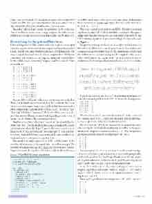
Figure 2 The CD-1 Training Algorithm
each RBM node value can be zero or one, with three hidden nodes there are a total of eight people types that can be detected: (0, 0, 0),(0,0,1),...(1,1,1).
There are several ways to train an RBM. The most common algorithm is called CD-1, which stands for contrastive divergence, single-step. The algorithm is very clever and isn’t at all obvious. The CD-1 training algorithm is presented in high-level pseudo-code in Figure 2.
The goal of training is to find a set of weights and bias values so that when the RBM is fed a set of input values in the visible nodes and generates a set of output nodes in the hidden nodes, then when the hidden nodes are used as inputs, the original visible nodes values will (usually) be regenerated. The only way I was able to understand CD-1 was by walking through a few concrete examples.
Determining a set of RBM output values for a given set of input values is easy, but where do the weights and bias values come from?
Suppose the learning rate is set to 0.01 and that at some point the
current training input item is (0, 0, 1, 1, 0, 0) and the 18 weights are:
0.01 0.02 0.03 0.04 0.05 0.06 0.07 0.08 0.09 0.10 0.11 0.12 0.13 0.14 0.15 0.16 0.17 0.18
The row index, 0 to 5, represents the index of a visible node and the column index, 0 to 2, represents the index of a hidden node. So the weight from visible[0] to hidden[2] is 0.03.
The first step in CD-1 is to compute the h values from the v values using the probabilistic mechanism described in the previ- ous section. Suppose h turns out to be (0, 1, 0). Next, the positive
gradient is computed as the outer product of v and h:
000 000 010 010 000 000
The outer product isn’t very common in machine learning algo- rithms (or any other algorithms for that matter), so it’s quite possible you haven’t seen it before. The Wikipedia article on the topic gives a pretty good explanation. Notice that the shape of the positive gradient matrix will be the same as the shape of the weight matrix.
Next, the h values are used as inputs, along with the current weights, to produce new output values v'. Suppose v' turns out to be (0, 1, 1, 1, 0, 0). Next, v' is used as the input to compute a new h'. Suppose h' is (0, 0, 1).
The negative gradient is the outer product of v' and h' and so is:
000 001 001 001 000 000
(v represents the visible nodes) (h represents the hidden nodes) (lr is a small learning rate value)
loop n times
for each data item
compute h from v
let posGrad = outer product(v, h) compute v' from h
compute h' from v'
let negGrad = outer product(v', h') let delta W = lr * (posGrad - negGrad) let delta vb = lr * (v - v')
let delta hb = lr * (h - h')
end for end loop
msdnmagazine.com
June 2017 55