Page 67 - MSDN Magazine, November 2019

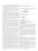
variation of mixture model clustering and EM optimization used in this article are shown in Figure 2. Depending on your math background, the equations may appear intimidating, but they’re actually quite simple, as you’ll see shortly.
The key to the variation of mixture model clustering presented here is understanding the multivariate Gaussian (also called normal) probability distribution. And to understand the multi- variate Gaussian distribution, you must understand the univariate Gaussian distribution.
Suppose you have a dataset that consists of the heights (in inches) of men who work at a large tech company. The data would look like 70.5, 67.8, 71.4 and so forth (all inches). If you made a bar graph for the frequency of the heights, you’d likely get a set of bars where the highest bar is for heights between 68.0 to 72.0 inches (frequen- cy about 0.6500). You’d get slightly lower bars for heights between 64.0 to 68.0 inches, and for 72.0 inches to 76.0 inches (about 0.1400 each), and so on. The total area of the bars would be 1.0. Now if you drew a smooth line connecting the tops of the bars, you’d see a bell-shaped curve.
The univariate Gaussian distribution is a mathematical abstrac- tion of this idea. The exact shape of the bell-shaped curve is determined by the mean (average) and variance (measure of spread). The math equation that defines the bell-shaped curve of a univariate Gaussian distribution is called the probability densi- ty function (PDF). The math equation for the PDF of a univariate Gaussian distribution is shown as equation (1) in Figure 2. The variance is given by sigma squared. For example, if x = 1.5, u = 0, and var = 1.0 then f(x, u, var) = 0.1295, which is the height of the bell-shaped curve at point x = 1.5.
The value of the PDF for a given value of x isn’t a probability. The probability of a range of values for x is the area under the curve of the PDF function, which can be determined using calculus. Even though a PDF value by itself isn’t a probability, you can compare PDF values to get relative likelihoods. For example, if PDF(x1) = 0.5000 and PDF(x2) = 0.4000 you can conclude that the proba- bility of x1 is greater than the probability of x2.
Now, suppose your dataset has items where each has two or more values. For example, instead of just the heights of men, you have (height, weight, age). The math abstraction of this scenario is called the multivariate Gaussian distribution. The dimension, d, of a multivariate Gaussian distribution is the number of values in each data item, so (height, weight, age) data has dimension d = 3.
The equation for the PDF of a multivariate Gaussian distribution is shown as equation (2) in Figure 2. The x is in bold to indicate it’s a multivalued vector. For a multivariate Gaussian distribution, instead of a variance, there is a (d x d) shape covariance matrix, represented by Greek letter uppercase sigma. Calculating the PDF for a univariate x is simple, but calculating the PDF for a mul- tivariate x is extremely difficult because you must calculate the determinant and inverse of a covariance matrix.
Instead of using the multivariate Gaussian distribution, you can greatly simplify mixture model calculations by assuming that each component of a multivalued data item follows an independent univariate Gaussian distribution. For example, suppose d = 3 and x = (0.4, 0.6, 0.8). Instead of calculating a multivalued mean and msdnmagazine.com
Figure 2 Mixture Model Expectation-Maximization Optimization Equations
a (d x d) multivalued covariance matrix and then using equation (2), you can look at each data component separately. This would give you three means, each a single value, and three variances, each also a single value. Then you can calculate three separate PDF values using equation (1) and average the three PDF values to get a final PDF value.
This technique is called a Gaussian mixture model because it assumes the data is clustered according to a mixture of K multi- variate Gaussian probability distributions. It’s known as a naive approach because the assumption that the data components are mathematically independent of each other is rarely true for real-life data. However, the naive Gaussian PDF approach is dra- matically simpler than calculating a true multivariate Gaussian PDF, and the naive technique often (but not always) works well in practice.
The Demo Program
The complete demo program, with several minor edits to save space, is presented in Figure 3. To create the program, I launched Visual Studio and created a new console application named MixtureModel. I used Visual Studio 2017, but the demo has no significant .NET Framework dependencies.
After the template code loaded, at the top of the editor window I removed all unneeded namespace references, leaving just the ref- erence to the top-level System namespace. In the Solution Explorer window, I right-clicked on file Program.cs, renamed it to the more descriptive MixtureModelProgram.cs and allowed Visual Studio to automatically rename class Program.
All normal error checking has been omitted to keep the main ideas as clear as possible. I used static methods and class-scope constants rather than OOP for simplicity.
November 2019 55