Page 48 - MSDN Magazine, May 2019

it. Here, I’ll use the following two-parameter Weibull distribution version for t>=0:
ƒ(t) = λktk-1e-λtk
(There are also versions with three parameters.) The two parame- ters of the distribution are the shape that’s determined by k and the scale that’s determined by lambda. A rough analogy is the way a bell- shaped distribution has a characteristic mean and standard deviation.
Recall that the relationship between the distribution density function f(t), the hazard function h(t) and the survival function s(t) is given by f(t) = h(t)s(t).
The following are the Weibull hazard and survival functions:
h(t) = λktk-1
s(t) = e-λtk
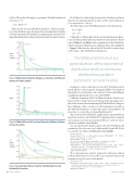
Unlike the Cox PH model, both the survival and the hazard func- tions are fully specified and have parametric representations. Please refer to Figure 3 and Figure 4 for visualizations of the Weibull dis- tribution and survival functions for different values of k and lambda.
Figure 5 illustrates the effects that AFT model covariates have on the shape of the Weibull survival function.
The Weibull distribution is a generalization of the exponential distribution and is a continuous distribution popular in parametric survival models.
Estimation of the coefficients for the AFT Weibull model in Spark MLLib is done using the maximum likelihood estimation algorithm. You can learn more about how it’s done at bit.ly/2XSauom, and find the implementation code at bit.ly/2HtJw0v.
Unlike the estimation of the Cox PH model, where only the coef- ficients of the covariates are reported (along with some diagnostics), the results obtained from estimating the Weibull AFT model report the coefficients of the covariates, as well as parameters specific for the Weibull distribution—an intercept and a scale parameter. I’ll show how to convert those to k and lambda in a bit.
The results for the Weibull AFT implementation in Spark MLLib match the results for the Weibull AFT implementation using the survreg function from the popular R library “survival” (more details are available at bit.ly/2XSxkw8).
You can run the following R script for the AFT Weibull model estimation (the code runs on a locally installed Spark MLLi, but you can also use Spark on HDInsight at bit.ly/2u2U5Qf):
library(survival)
library(SparkR, lib.loc = c(file.path(Sys.getenv("SPARK_HOME"), "R", "lib"))) sparkR.session(master = "local[*]")
inputFileName<-'comp1_df.csv'
df<-read.csv(inputFileName, header=TRUE, stringsAsFactors=TRUE) aftMachineDF<-suppressWarnings(createDataFrame(df))
aftMachineModel <- spark.survreg(aftMachineDF,Surv(time_to_event, event) ~ model +
age_mean_centered + volt_mean_centered + rotate_mean_centered +
pressure_mean_centered + vibration_mean_centered) summary(aftMachineModel)
The script generates only the estimated coefficients without additional information. It’s possible to get such information by running survreg (because results match):
library(survival)
machineModel<-survreg(Surv(time_to_event, event) ~ model + age_mean_centered +
volt_mean_centered+rotate_mean_centered + pressure_mean_centered +
vibration_mean_centered, df, dist='weibull') summary(machineModel)
1.0 0.8 0.6
K=10, lambda = 1
Weibull Survival Probability
Figure 3 Weibull Distribution Shape as a Function of Different Values of K and Lambda
K=1, lambda =1
0.4 K=1,
lambda = 0.5
0.2
0.0
0 2 4 6 8 10
t
3.5 3.0 2.5
Weibull 2.0 1.5
K=10, lambda = 1
K=1,
lambda 1.0 = 1
0.5
K=1,
lambda = 0.5
0.0
0 2 4 6 8 10
t
Figure 4 Weibull Survival Function Shape for Different Values of K and Lambda
AFT Weibull Survival Probability
1.0 0.8 0.6 0.4 0.2
K=1,
lambda = 0.5,
acceleration factor of exp(-1)
K=1,
lambda = 0.5, baseline
K=1,
lambda = 0.5, acceleration factor of exp(1)
0.0
0 2 4 6 8 10
t
Figure 5 Accelerated Failure Time for the Weibull Survival Probability Function
42 msdn magazine
Machine Learning