Page 47 - MSDN Magazine, May 2019

With the Cox PH model specified, the coefficients and the non-parametric baseline hazard can be estimated using various techniques. One popular technique is partial maximum likelihood estimation (also used in h2o.ai).
The following code snippet is an R script that runs an estimation of the Cox PH model using h2o.ai on the mean centered covari- ates (machine telemetry and age) and the categorical covariate machine model:
library(h2o)
localH2O <- h2o.init()
inputFileName<-'comp1_df.csv'
df<-read.csv(inputFileName, header=TRUE, stringsAsFactors=TRUE)
df.hex <- as.h2o(df, key = "df.hex")
model <- h2o.coxph(x = c("age_mean_centered", "model","volt_mean_centered",
"rotate_mean_centered","pressure_mean_centered", "vibration_mean_centered"),
event_column = "event", stop_column ="time_to_event" ,training_frame = df.hex) summary(model)
At the time of this writing, the Cox PH model in h2o.ai isn’t available to use from Python, so R code is provided. Installation instructions are available at bit.ly/2z2QweL, or, for h2o.ai with Azure HDInsight, at bit.ly/2J7nXp6.
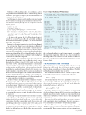
Running the code snippet generates the output shown in Figure 2.
The first important thing to note is the estimated coefficients of the covariates. The machine model covariate is encoded as a cate- gorical data type. The baseline for this category is model1, which is represented by setting the three covariates encoding the other three machine models (model.model2, model.model3 and model.model4) to zero. Each covariate gets its own coefficient. Understanding how to interpret the coefficients is important.
If you apply the exponential function to the coefficients for the machine model covariates (exp(coeff ) in the output), you see that model.model2 has a value of 0.9352, while model.model4 has a value of 1.3619. This means that machines of model2 have a hazard rate that’s 6.5 percent lower than the hazard rate of the baseline machine model (model 1), and that machines of model. model4 have a considerably higher hazard of 36.2 percent com- pared to machines of model.model1. In other words, machines of model.model4 have the highest risk of failure, while machines of model.model2 have the lowest risk of failure. Therefore, when pri- oritizing maintenance operations, the model of the machine should be an important factor to take into consideration.
All other covariates are mean centered continuous covariates. The interpretation of the coefficients affiliated with them is that now the hazard ratio is given by the exponential of the covariates around their means. Therefore, by increasing a covariate value by one unit (keeping all other covariates fixed), the hazard ratio increases (or decreases) by the exponential of the coefficient (in a similar way to that of the categorical variable). So, for example, by increasing the voltage by one unit, the risk for failure increases by 3.2 percent.
Another important point to mention here concerns model diag- nostics techniques. Such techniques provide a basis to understand whether the model considered (in this case, the Cox PH model) is appropriate. Here, the Rsquare value (a value between zero and one, the higher the better) is relatively low (0.094) and most of the z-scores of the coefficients don’t indicate that the coefficients are statistically significant (there isn’t enough evidence to support that they’re different from zero). Both of these indicators lead to msdnmagazine.com
Figure 2 Output for the Cox PH Regression
Surv(time_to_event, event) ~ model + volt_mean_centered + rotate_mean_centered + pressure_mean_centered + vibration_mean_centered + age_mean_centered
n= 709, number of events= 192
coef model.model2 -0.066955 model.model3 -0.021837 model.model4 0.308878 volt_mean_centered 0.031903 rotate_mean_centered 0.001632 pressure_mean_centered -0.008164 vibration_mean_centered 0.018220 age_mean_centered 0.004804
exp(coef) 0.935237 0.978400 1.361896 1.032418 1.001633 0.991869 1.018387 1.004815
se(coef) z 0.257424 -0.260 0.215614 -0.101 0.227469 1.358 0.003990 7.995 0.001362 1.199 0.005768 -1.415 0.013866 1.314 0.013293 0.361
Pr(>|z|) 0.795
0.919
0.174 1.33e-15 *** 0.231
0.157 0.189 0.718
---
Signif.codes: 0‘***’0.001‘**’0.01‘*’0.05‘.’0.1‘’1
model.model2 model.model3 model.model4 volt_mean_centered rotate_mean_centered pressure_mean_centered vibration_mean_centered age_mean_centered
exp(coef) exp(-coef) lower .95 upper .95 0.9352 1.0692 0.5647 1.549 0.9784 1.0221 0.6412 1.493 1.3619 0.7343 0.8720 2.127 1.0324 0.9686 1.0244 1.041 1.0016 0.9984 0.9990 1.004 0.9919 1.0082 0.9807 1.003 1.0184 0.9819 0.9911 1.046 1.0048 0.9952 0.9790 1.031
Rsquare= 0.094 (max possible= 0.941 )
Likelihood ratio test= 70.1 on 8 df, p=4.69e-12 Wald test = 70.19 on 8 df, p=4.514e-12
the conclusion that there’s room for improvement, for example through feature engineering. There are also other statistical tests that are specific to the Cox PH model that should be conducted. You can consult the survival analysis literature I mentioned earlier for more details.
The Accelerated Failure Time Model
The survival regression model in Spark MLLib is the Accelerated Failure Time (AFT) model. This model directly specifies a survival function from a certain theoretical math distribution (Weibull) and has the accelerated failure time property.
The AFT model is defined as follows. Assume an object is char- acterized by using the (linear) covariates and coefficients:
β1X1 +...+ βpXp
Also assume that the object has a parametric survival func- tion s(t) and, denoted by s0(t), the survival function of a baseline object (with all covariates set to zero). The AFT model defines the relationship between s(t) and s0(t) as:
S(t) = S0(teβ1 X1 +...+ βp Xp)
From this definition you can see why the model is called Accelerated Failure Time model. It’s because the survival function includes an accelerator factor, which is the exponential function of the linear combinations of the covariates, which multiplies the survival time t.
This type of model is useful when there are certain covariates, such as age (in my dataset, machine age), that may cause mono- tonic acceleration or deceleration of survival/failure time.
The Weibull distribution is a generalization of the exponential distribution and is a continuous distribution popular in parametric survival models. There are a few variations on how to parameterize
May 2019 41