Page 48 - MSDN Magazine, November 2018

To calculate max flex displacement, we can use angular velocity of the tip of the board or linear acceleration. Angular velocity will be out of phase with corresponding acceleration, however, because acceleration is the time derivative of velocity. The same relationship exists between displacement and velocity, because velocity is the time derivative of displacement. That means that velocity will be 0 at the max flexion (bottom point of displacement) of the diving board and acceleration is at max (Figure 2, Step 5). After that, the board goes to horizontal position where displacement equals 0 and velocity is max (Figure 2, Step 7). We calculated max flexion displacement angle by integrating angular velocity over time from our first point of zero (Figure 2, Step 5) to our second point of the takeoff where angular velocity becomes max (Figure 2, Step 7).
In our calculations we use the International System of Units (SI).
To start, in the R code (Figure 4) you can call the do-it-all func- tion that parses files and displays results, like so:
CalculateSpringBoardDivingValues (sourceFile,lag, threshold, influence,1)
Let’s dig into the details of what’s happening inside this call. First, the function loads data from the raw sensor file source into the data frame, with this code:
df <- ReadNewFormatFile(dat2, debug_print = debug_print)
Sensors like gyro and accelerometer use somewhat-specific data formats, mostly for data optimization purposes. For example, the gyroscope produces angular velocity values in millidegrees per second (mdps). This is done to avoid using floating-point num- bers. In our calculations we use the International System of Units (SI), used throughout most physics calculations. For acceleration, we also convert raw sensor values to m/s^2, a standard unit for acceleration. Here are the calculations:
Our drift, or error, is minimized because we only look at the moment when the springboard starts bouncing. In R, this is the code for our integration:
# Interested only in [posStart:posEnd]
# When displacement is at MAX, velocity passes 0 point revFirstMin <- which.min(rev(wSm$avgFilter[posStart:posEnd]))
# After been max negative
posLastMin <- posEnd - revFirstMin +1
# Next index when Angular Velocity goes
# through 0 is our starting integration point
nextZero <- min(which(floor(wSm$avgFilter[posLastMin:posEnd])>0)) # 0 position relative to Last Minimum
nextZero <- nextZero + posLastMin -1
# Max position after 0 position
nextMaxAfterZero <- which.max(wSm$avgFilter[nextZero:posEnd]) nextMaxAfterZero <- nextMaxAfterZero + nextZero -1
We also provided plotting functions to draw the results, as shown here:
PlotSingleChart(wSm$avgFilter[posStart:posEnd],
"Angular Velocity Smooth OUR Segment ","cyan4", kitSensorFile, "Wx smooth deg.",TRUE, FALSE, d$Start[posStart:posEnd])
In the charts on Figure 6, we plot data from the gyro sensor while the board is still, through the hurdle and after the takeoff moment. It’s clear that the board reaches its maximum amplitude before the takeoff, after which the oscillation diminishes with time. To make our calculation more precise, and minimize drift error from the integra- tion, we only use the moment between when the springboard starts oscillating to the moment when oscillation reaches its maximum.
Finally, we calculate the maximum flexion angle and the takeoff time, with this code:
timeTakeOff <- d$Start[posHorizontal] timeStart <- d$Start[posLastMin]
writeLines (paste (
"Hurdle landing time (Start) = ", timeStart,"\n",
"Take Off time (End) = ", timeTakeOff,"\n",
"Board contact time (from hurdle landing to takeoff) = ", round(difftime(
as.POSIXct(paste(dt,df$t[posHorizontal],sep=" ")), as.POSIXct(paste(dt,df$t[posLastMin],sep=" "))),digits = 4)," secs \n", "Maximum downward flexion of the board = ", round(max(abs(d$theta2Cum[posLastMin:nextZero])),digits=4)," deg.",
" secs", sep="" ))
Getting this sensor data is absolutely essential for diving coaches and athletes, as it provides them with valuable information about the dive, especially the takeoff component that’s so vital to a successful dive.
Video Capture and Analysis
Video Analysis Overview Currently, diving coaches rely heavily on what they see to give feedback to their divers. They need to be able to associate the data they receive from our sensors with what they see with their own eyes. By correlating sensor data with video, we give coaches the ability to better under- stand what they’re seeing.
Syncing sensor telemetry with captured video is actually a bit of a challenge. To do so, we turned to a computer vision library, called openCV, to visually determine the exact moment when the diver is at his lowest point, when the board is fully flexed just before take- off. We then synced that point on the video with the lowest measured point reported by
# wx, wy, wz *
# ax, at, az = df$wx <- df$wx * df$wy <- df$wy * df$wz <- df$wz * df$ax <- df$ax * df$ay <- df$ay * df$az <- df$az *
0.001 * degrees/second (ang. Velocity) * 0.001 * 9.81 = m/s^2 (acceleration)
0.001 # convert to degrees per second 0.001 # convert to degrees per second 0.001 # convert to degrees per second
0.001 * 9.81 0.001 * 9.81 0.001 * 9.81
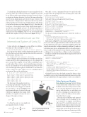
The direction of the angular velocity vec- tor points perpendicular to the plane of the motion, while rotation happens around the axis of rotation, as shown in Figure 5. We can determine the axis of rotation by the axis with the most significant value change. A little math here, for angular velocity is the rate of change of the angle over time:
ω= d0 dt
To obtain the angle, we can simply inte- grate angular velocity over time:
t
42 msdn magazine
Artificial Intelligence
ω(t) = ∫t w(t) dt ≈∑ω(t) Ts 0 0
Figure 5 Gyroscope-Sensing Angular Orientation