Page 26 - MSDN Magazine, April 2018

the DataFrame to just six. While the original dataset has a column indicating if a flight was delayed 15 minutes or more, I would like to add some more granularity. I’ll create a new column set to 1 if a flight is delayed 10 minutes or more and name that column “IsDelayed.” Additionally, I call the dropna function, which drops any rows with null values. ML algorithms can be finicky about the data inputs they receive. Very often an unexpected null value will throw an exception, or worse, corrupt the results. Enter the fol- lowing code into a new cell and execute it. The results will show the first 20 rows of model_data:
model_data = flights_df.select("DAY_OF_MONTH", "DAY_OF_WEEK", "ORIGIN_AIRPORT_ID", "DEST_AIRPORT_ID", "DEP_DELAY", ((col("ARR_DELAY") > 10).cast("Int").alias("IsDelayed"))).dropna()
model_data.show()
Supervised Learning
In supervised ML, the ground truth is known. In this case, it’s the on-time arrival records of flights in the United States for June 2015. Based on that data, the algorithm will generate a predictive model on whether a flight’s arrival will be delayed by 10 minutes or more given the five fields: Day of Month, Day of Week, Origin Airport ID, Destination Airport ID and Departure Delay. In ML terms, those fields are collectively referred to as “features.” The predicted value, in this case an indicator of an arrival delay of 10 minutes or less than 10 minutes, is referred to as the “label.”
Supervised ML models are often tested with the same dataset on which they’re trained. To do this, they’re randomly split into two datasets: one for training and one for testing. Usually, they’re split along a 60/40 or 70/30 line with the larger share going into the training data.
The following code separates the training data and the test data into two sets along a 70/30 line and displays the count (once again, enter the code into a new cell and execute it):
split_model_data = model_data.randomSplit([0.7,0.3]) training_data = split_model_data[0]
testing_data = split_model_data[1]
all_data_count = training_data.count() + testing_data.count()
print ("Rows in Training Data: " + str(training_data.count())) print ("Rows in Testing Data: " + str(testing_data.count())) print ("Total Rows: " + str(all_data_count))
There will be a discrepancy in the total rows displayed here and ear- lier in the notebook. That’s due to rows with null values being dropped.
The test data now must be further modified to meet the require- ments of the ML algorithm. The five fields representing the features will be combined into an array, or a vector, through a process called vectorization. The IsDelayed column will be renamed to label. The training DataFrame will have just two columns: features and label. Enter the following code into an empty cell and execute it and the first 20 rows of the training DataFrame will be displayed:
vector_assembler = VectorAssembler(
inputCols = ["DAY_OF_MONTH", "DAY_OF_WEEK", "ORIGIN_AIRPORT_ID", "DEST_AIRPORT_ID", "DEP_DELAY"], outputCol="features")
training = vector_assembler.transform(training_data).select(col("features"), col("IsDelayed").cast("Int").alias("label")) training.show(truncate=False)
Supervised ML models are often tested with the same dataset on which they’re trained.
With the training data split into two columns, features and labels, it’s ready to be fed to the ML algorithm. In this case, I’ve cho- sen logistic regression. Logistic regression is a statistical method for analyzing data where one or more input variables influence an outcome. For this model, the input variables are the contents of the feature column, the fields DAY_OF_MONTH, DAY_OF_WEEK, ORIGIN_AIRPORT_ID, DEST_AIRPORT_ID and DEP_DELAY. The outcome is the label column, or if the flight was delayed more than 10 minutes. This algorithm will not distinguish between a delay of 10 minutes and one second and a 15-hour delay. The model is created by fitting the training data to it. Again, enter the follow- ing code into a blank cell and execute it:
logR = LogisticRegression(labelCol="label", featuresCol="features", maxIter=10, regParam=0.1)
model = logR.fit(training)
With the model trained, the only thing left to do is test it. The testing data must also be modified to fit the expectations of the algorithm by running it through the vector assembler as the training data was. Enter the following code into a blank cell and execute it:
testing = vector_assembler.transform(testing_data).select(col("features"), (col("IsDelayed")).cast("Int").alias("trueLabel"))
testing.show()
Now that the training data is prepared, the next step is to run it through the model by calling the transform method. The output is a DataFrame with four col- umns: the features, the predicted value, the actual value and the probability, a measure of how confident the algorithm was in its prediction. Once more, enter the following code into an empty cell and execute it:
prediction = model.transform(testing) predicted = prediction.select("features", "prediction", "trueLabel", "probability") predicted.show()
The output only shows the first 20 rows. That’s not an efficient way of measuring
Artificially Intelligent
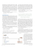
Figure 6 Creating a New PySpark 3 Jupyter Notebook 20 msdn magazine