Page 67 - MSDN Magazine, March 2018

The first step is to deal with missing data—notice the “?” in item [303]. Because there are only six items with missing values, those six items were just tossed out, leaving 297 items.
The next step is to normalize the numeric predictor values, such as age in the first column. The demo used min-max normalization where the value in a column is replaced by (value - min) / (max - min). For example, the minimum age value is 29 and the max- imum is 77, so the first age value, 63, is normalized to (63 - 29) / (77-29)=34/48=0.70833.
The next step is to encode the categorical predictor values, such as sex (0 = female, 1 = male) in the second column and pain type (1, 2, 3, 4) in the third column. The demo used 1-of-(N-1) encoding so sex is encoded as female = -1, male = +1. Pain type is encoded as 1=(1,0,0),2=(0,1,0),3=(0,0,1),4=(-1,-1,-1).
The last step is to encode the value to predict. When using a neu- ral network for binary classification, you can encode the value to predict using just one node with a value of 0 or 1, or you can use two nodes with values of (0, 1) or (1, 0). For a reason I’ll explain shortly, when using CNTK, it’s much better to use the two-node technique. So, 0 (no heart disease) was encoded as (0, 1) and values 1 through 4 (heart disease) were encoded as (1, 0).
The final normalized and encoded data was tab-delimited and looks like:
|symptoms 0.70833 1 1 0 0 0.48113 ... |disease 0 1 |symptoms 0.79167 1 -1 -1 -1 0.62264 ... |disease 1 0 ...
Tags “|symptoms” and “|disease” were inserted so the data could be easily read by a CNTK data reader object.
The Demo Program
The complete demo program, with a few minor edits to save space, is presented in Figure 3. All normal error checking has been removed. I indent with two space characters instead of the usual four as a matter of personal preference and to save space. The “\” character is used by Python for line continuation.
The cleveland_bnn.py demo has one helper function, create_ reader. All control logic is in a single main function. Because CNTK is young and under vigorous development, it’s a good idea to add a comment detailing which version is being used (2.3 in this case).
Installing CNTK can be a bit tricky. First, you install the Anaconda distribution of Python, which contains the required Python inter- preter, required packages such as NumPy and SciPy, and useful utilities such as pip. I used Anaconda3 4.1.1 64-bit, which includes Python 3.5. After installing Anaconda, you install CNTK as a Python package, not as a standalone system, using the pip utility. From an ordinary shell, the command I used was:
>pip install https://cntk.ai/PythonWheel/CPU-Only/cntk-2.3-cp35-cp35m-win_amd64.whl
Almost all CNTK installation failures I’ve seen have been due to Anaconda-CNTK version incompatibilities.
The demo begins by preparing to create the neural network:
input_dim = 18
hidden_dim = 20
output_dim = 2
train_file = ".\\Data\\cleveland_cntk_twonode.txt"
X = C.ops.input_variable(input_dim, np.float32) Y = C.ops.input_variable(output_dim, np.float32)
The number of input and output nodes is determined by your data, but the number of hidden processing nodes is a free parameter and must be determined by trial and error. Using 32-bit variables is typical for neural networks because the precision gained by using 64 bits isn’t worth the performance penalty incurred.
The network is created like so:
with C.layers.default_options(init=C.initializer.uniform(scale=0.01,\ seed=1)):
hLayer = C.layers.Dense(hidden_dim, activation=C.ops.tanh,
name='hidLayer')(X)
oLayer = C.layers.Dense(output_dim, activation=None,
name='outLayer')(hLayer) nnet = oLayer
model = C.ops.softmax(nnet)
The Python with statement is a syntactic shortcut to apply a set of common arguments to multiple functions. The demo uses tanh activation on the hidden layer nodes; a common alternative is the sigmoid function. Notice that there’s no activation applied to the output nodes. This is a quirk of CNTK because the CNTK training function expects raw, un-activated values. The nnet object is just a convenience alias. The model object has softmax activation so it can be used after training to make predictions. Because Python assigns by reference, training the nnet object also trains the mode object.
Training the Neural Network
The neural network is prepared for training with:
tr_loss = C.cross_entropy_with_softmax(nnet, Y) tr_clas = C.classification_error(nnet, Y) max_iter = 5000
batch_size = 10
learn_rate = 0.005
learner = C.sgd(nnet.parameters, learn_rate)
trainer = C.Trainer(nnet, (tr_loss, tr_clas), [learner])
The tr_loss (“training loss”) object tells CNTK how to measure error when training. An alternative to cross entropy with softmax is squared error. The tr_clas (“training classification error”) object can be used to automatically compute the percentage of incorrect predictions during or after training.
The values for the maximum number of training iterations, the number of items in a batch to train at a time, and the learning rate, are all free parameters that must be determined by trial and error. You can think of the learner object as an algorithm, and the trainer object as the object that uses the learner to find good values for the neural network’s weights and biases.
March 2018 61
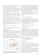
210 190 170 150 130 110
90 70 50
Cleveland Heart Disease
No Disease Disease
20 30 40 50 60 70 80 Age
Figure 2 Cleveland Heart Disease Partial Raw Data msdnmagazine.com
Blood Pressure