Page 66 - MSDN Magazine, March 2018

TesT Run JAMES MCCAFFREY Neural Binary Classification Using CNTK
n e
The goal of a binary classification problem is to make a prediction where the value to predict can take one of just two possible values. For example, you might want to predict if a hospital patient has heart disease or not, based on predictor variables such as age, blood pressure, sex and so on. There are many techniques that can be used to tackle a binary classification problem. In this article I’ll explain how to use the Microsoft Cognitive Toolkit (CNTK) library to create a neural network binary classification model.
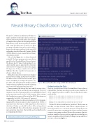
Take a look at Figure 1 to see where this article is headed. The demo program creates a prediction model for the Cleveland Heart Disease dataset. The dataset has 297 items. Each item has 13 pre- dictor variables: age, sex, pain type, blood pressure, cholesterol, blood sugar, ECG, heart rate, angina, ST depression, ST slope, number of vessels and thallium. The value to predict is the presence or absence of heart disease.
Behind the scenes, the raw data was normalized and encoded, resulting in 18 predictor variables. The demo creates a neural network with 18 input nodes, 20 hidden processing nodes and two out- put nodes. The neural network model is trained using stochastic gradient descent with a learning rate set to 0.005 and a mini-batch size of 10.
Figure 1 Binary Classification Using a CNTK Neural Network
During training, the average loss/error and the average classi- fication accuracy on the current 10 items is displayed every 500 iterations.Youcanseethat,ingeneral,loss/errorgraduallydecreased and accuracy increased over the 5,000 iterations. After training, the classification accuracy of the model on all 297 data items was computed to be 84.18% (250 correct, 47 incorrect).
This article assumes you have intermediate or better program- ming skill, but doesn’t assume you know much about CNTK or neural networks. The demo is coded using Python, but even if you don’t know Python, you should be able to follow along without too much difficulty. The code for the demo program is presented in its entirety in this article. The data file used is available in the accompanying download.
Understanding the Data
There are several versions of the Cleveland Heart Disease dataset at bit.ly/2EL9Leo. The demo uses the processed version, which has 13 of the original 76 predictor variables. The raw data has 303 items and looks like:
[001] 63.0,1.0,1.0,145.0,233.0,1.0,2.0,150.0,0.0,2.3,3.0,0.0,6.0,0 [002] 67.0,1.0,4.0,160.0,286.0,0.0,2.0,108.0,1.0,1.5,2.0,3.0,3.0,2 [003] 67.0,1.0,4.0,120.0,229.0,0.0,2.0,129.0,1.0,2.6,2.0,2.0,7.0,1 ...
[302] 57.0,0.0,2.0,130.0,236.0,0.0,2.0,174.0,0.0,0.0,2.0,1.0,3.0,1 [303] 38.0,1.0,3.0,138.0,175.0,0.0,0.0,173.0,0.0,0.0,1.0,?,3.0,0
The first 13 values in each line are predictors. The last item in each line is a value between 0 and 4 where 0 means absence of heart disease and 1, 2, 3, or 4 means presence of heart disease. In general, the most time-consuming part of most machine learning scenarios is preparing your data. Because there are more than two predictor variables, it’s not possible to graph the raw data. But you can get a rough idea of the problem by looking at just age and blood pressure, as shown in Figure 2.
Code download available at msdn.com/magazine/0318magcode.
60 msdn magazine