Page 71 - MSDN Magazine, November 2017

The RBF function is best explained by example. Suppose v1 = (3.0, 1.0, 2.0) and v2 = (1.0, 0.0, 5.0), and sigma is 1.5. First, you compute the squared Euclidean distance:
||v1-v2||^2=(3.0-1.0)^2+(1.0-0.0)^2 +(2.0-5.0)^2 =4.0+1.0+9.0
= 14.0
Next, you divide the squared distance by 2 times sigma squared:
14.0/(2*(1.5)^2)=14.0/4.5=3.11
Last, you take Euler’s number and raise it to the negative of the
previous result:
K(v1, v2) = e^(-3.11) = 0.0446
The small kernel value indicates that v1 and v2 are not very sim- ilar. The demo program defines the RBF kernel function as:
static double Kernel(double[] v1, double[] v2, double sigma)
{
double num = 0.0;
for (int i = 0; i < v1.Length - 1; ++i)
num += (v1[i] - v2[i]) * (v1[i] - v2[i]); double denom = 2.0 * sigma * sigma;
double z = num / denom;
return Math.Exp(-z);
}
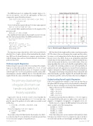
9.0 8.0 7.0 6.0 5.0 4.0 3.0 2.0 1.0 0.0
0.0 1.0
Dummy Training and Test Data for KLR
0
1 Test
The function assumes that the last cell of each array holds the class label (0 or 1) and so the last cell isn’t included in the calcula- tion. KLR uses the kernel function to compare a given data item with all training items, and uses that information to determine a predicted class label.
Ordinary Logistic Regression
Ordinary logistic regression (LR) is best explained by example. Suppose you have three predictor variables: x0 = 2.5, x1 = 1.7, and x2 = 3.4. A regular LR model creates a set of numeric constants called weights (wi), one for each predictor variable, and an addi- tional numeric constant called the bias (b). Note that the bias in regular LR isn’t the same as the KLR bias shown in Figure 1.
The primary disadvantage of regular LR is that it can handle only data that’s linearly separable.
Suppose w0 = 0.11, w1 = 0.33, w2 = 0.22, b = 0.44. To predict the class label, 0 or 1, for the input data (2.5, 1.7, 3.4) you first com- pute the sum of the products of each x and its associated w, and add the bias:
z = (2.5)(0.11) + (1.7)(0.33) + (3.4)(0.22) + 0.44 = 2.024
Next, you compute p = 1.0 / (1.0 + exp(-z)): p = 1.0 / (1.0 + exp(-2.024))
= 0.8833
The p value is the probability that the data item has class label =
1, so if p is less than 0.5, your prediction is 0 and if p is greater than 0.5 (as it is in this example), your prediction is 1. msdnmagazine.com
OK, but where do the weights and bias values come from in regular LR? The idea is that you determine the weights and bias values by using a set of training data that has known input values and known, correct class labels, then use an optimization algorithm to find values for the weights and biases so that the predicted class labels closely match the known, correct label values. There are many algorithms that can be used to find the weight and bias values for regular LR, including gradient ascent with log likelihood, gradient descent with squared error, iterated Newton-Raphson, simplex optimization, L-BFGS and particle swarm optimization.
The primary disadvantage of regular LR is that it can handle only data that’s linearly separable. Regular LR can’t handle data that’s not linearly separable, such as the demo data shown in Figure 2.
Understanding Kernel Logistic Regression
KLR is best explained by example. Let me state up front that at first glance KLR doesn’t appear very closely related to ordinary LR. However, the two techniques are closely related mathematically.
Suppose there are just four training data items: td[0] = (2.0, 4.0, 0)
td[1] = (4.0, 1.0, 1)
td[2] = (5.0, 3.0, 0)
td[3] = (6.0, 7.0, 1)
Your goal is to predict the class label for x = (3.0, 5.0). Suppose
the trained KLR model gave you alpha values and a bias of: alpha[0] = -0.3, alpha[1] = 0.4, alpha[2] = -0.2, alpha[3] =0.6, b = 0.1. The first step is to compute the RBF similarity between the data
item to predict each of the training items: K(td[0], x) = 0.3679
K(td[1], x) = 0.0002
K(td[2], x) = 0.0183
K(td[3], x) = 0.0015
Notice that at this point, x is most similar to td[0] and td[2], which
both have class label 0. Next, you compute the sum of products of each K value and the associated alpha, and add the bias value:
November 2017 67
2.0 3.0 4.0
5.0 6.0 7.0
8.0 9.0
Figure 2 Kernel Logistic Regression Training Data
x0
x1