Page 68 - MSDN Magazine, October 2017

TesT Run JAMES MCCAFFREY
Time-Series Regression Using a C# Neural Network
The goal of a time-series regression problem is to make predictions based on historical time data. For example, if you have monthly sales data (over the course of a year or two), you might want to predict sales for the upcoming month. Time-series regression is usually very difficult, and there are many different techniques you can use.
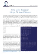
In this article, I’ll demonstrate how to perform a time-series regression analysis using rolling-window data combined with a neural network. The idea is best explained by an example. Take a look at the demo program in Figure 1. The demo program ana- lyzes the number of airline passengers who traveled each month between January 1949 and December 1960.
The demo data comes from a well-known benchmark dataset that you can find in many places on the Internet and is included with the download that accompanies this article. The raw data looks like:
"1949-01";112 "1949-02";118 "1949-03";132 "1949-04";129 "1949-05";121 "1949-06";135 "1949-07";148 "1949-08";148 ... "1960-11";390 "1960-12";432
There are 144 raw data items. The first field is the year and month. The second field is the total number of international airline passen- gers for the month, in thousands. The demo creates training data using a rolling window of size 4 to yield 140 training items. The training data is normalized by dividing each passenger count by 100:
[ 0] 1.12 1.18 1.32 1.29 1.21 [ 1] 1.18 1.32 1.29 1.21 1.35 [ 2] 1.32 1.29 1.21 1.35 1.48 [ 3] 1.29 1.21 1.35 1.48 1.48 ...
[139] 6.06 5.08 4.61 3.90 4.32
Notice that the explicit time values in the data are removed. The first window consists of the first four passenger counts (1.12, 1.18, 1.32, 1.29), which are used as predictor values, followed by the fifth count (1.21), which is a value to predict. The next window consists of the second through fifth counts (1.18, 1.32, 1.29, 1.21), which are the next set of predictor values, followed by the sixth count (1.35), the value to predict. In short, each set of four consecutive passen- ger counts is used to predict the next count.
The demo creates a neural network with four input nodes, 12 hid- den processing nodes and a single output node. The number of input
nodes corresponds to the number of predictors in the rolling window. The window size must be determined by trial and error, which is the biggest drawback to this technique. The number of neural network hidden nodes must also be determined by trial and error, which is always true for neural networks. There’s just one output node because time-series regression predicts one time unit ahead.
The neural network has (4 * 12) + (12 * 1) = 60 node-to-node weights and (12 + 1) = 13 biases, which essentially define the neural network model. Using the rolling-window data, the demo program trains the network using the basic stochastic back-propagation algorithm with a learning rate set to 0.01 and a fixed number of iterations set to 10,000.
Code download available at msdn.com/magazine/1017magcode.
64 msdn magazine
Figure 1 Rolling-Window Time-Series Regression Demo