Page 56 - MSDN Magazine, March 2019

new to Python, be aware that installing and managing add-on package dependencies is non-trivial.
After installing Python via the Anaconda distribution, the PyTorch package can be installed using the pip utility function with a .whl (“wheel”) file. PyTorch comes in a CPU-only version and in a GPU version. I used the CPU-only version.
Understanding the Data
The Boston Housing dataset comes from a research paper written
in 1978 that studied air pollution. You can find different versions of
the dataset in many locations on the Internet. The first data item is:
0.00632, 18.00, 2.310, 0, 0.5380, 6.5750, 65.20 4.0900, 1, 296.0, 15.30, 396.90, 4.98, 24.00
Each data item has 14 values and represents one of 506 towns near Boston. The first 13 numbers are the values of predictor vari- ables and the last value is the median house price in the town (divided by 1,000). Briefly, the 13 predictor variables are: crime rate in the town, large lot percentage, percentage zoned for industry, adjacency to Charles River, pollution, average number rooms per house, house age information, distance to Boston, accessibility to highways, tax rate, pupil-teacher ratio, proportion of Black resi- dents, and percentage of low-status residents.
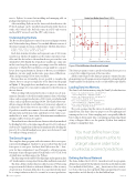
Because there are 14 variables, it’s not possible to visualize the dataset, but you can get a rough idea of the data from the graph in Figure 2. The graph shows median house price as a function of the percentage of town zoned for industry for the 102 items in the test dataset.
When working with neural networks, you must encode non- numeric data and you should normalize numeric data so that large values, such as a pupil-teacher ratio of 20.0, don’t overwhelm small values, such as a pollution reading of 0.538. The Charles River vari- able is a categorical value stored either as 0 (town is not adjacent) or 1 (adjacent). Those values were re-encoded as -1 and +1. The other 12 predictor variables are numeric. For each variable, I computed the min value and the max value, and then for every value x, nor- malized it as (x - min) / (max - min). After min-max normalization, all values will be between 0.0 and 1.0.
The median house values in the raw data were already normalized by dividing by 1,000, so the values ranged from 5.0 to 50.0, with most at about 25.0. I applied an additional normalization by dividing the prices by 10 so that all median house prices were between 0.5 and 5.0, with most being around 2.5.
The Demo Program
The complete demo program, with a few minor edits to save space, is presented in Figure 3. I indent two spaces rather than the usual four spaces to save space. And note that Python uses the ‘\’ char- acter for line continuation. I used Notepad to edit my program, but many of my colleagues prefer Visual Studio or VS Code, both of which have excellent support for Python.
ThedemoimportstheentirePyTorchpackageandassignsitanalias of T. An alternative is to import just the modules and functions needed. The demo defines a helper function called accuracy. When using a regression model, there’s no inherent definition of the accuracy of a prediction. You must define how close a predicted value must be to a target value in order to be counted as a correct prediction.
60 50 40 30 20 10
0
Boston Area Median House Prices (~1970)
0 5 10 15 20 25 30 Percentage Land Zoned for Industry
50 msdn magazine
Test Run
Figure 2 Partial Boston Area House Dataset
The demo program counts a predicted median house price as correct if it’s within 15 percent of the true value.
All the control logic for the demo program is contained in a sin- gle main function. Program execution begins by setting the global NumPy and PyTorch random seeds so results will be reproducible.
Loading Data into Memory
The demo loads data in memory using the NumPy loadtxt function:
train_x = np.loadtxt(train_file, delimiter="\t", usecols=range(0,13), dtype=np.float32)
train_y = np.loadtxt(train_file, delimiter="\t", usecols=[13], dtype=np.float32)
test_x = np.loadtxt(test_file, delimiter="\t", usecols=range(0,13), dtype=np.float32)
test_y = np.loadtxt(test_file, delimiter="\t", usecols=[13], dtype=np.float32)
The code assumes that the data is located in a subdirectory named Data. The demo data was preprocessed by splitting it into training and test sets. Data wrangling isn’t conceptually difficult, but it’s almost always quite time-consuming and annoying. Many of my colleagues like to use the pandas (Python data analysis) package to manipulate data.
You must define how close
a predicted value must be to a target value in order to be counted as a correct prediction.
DefiningtheNeuralNetwork
The demo defines the 13-(10-10)-1 neural network in a program- defined class named Net that inherits from the nn.Module module. YoucanthinkofthePython__init__functionasaclassconstruc- tor. Notice that you don’t explicitly define an input layer because input values are fed directly to the first hidden layer.
Median Price (x$1,000)