Page 44 - MSDN Magazine, March 2019

Training an SVM classifier is an iterative process and method Train returns the actual number of iterations that were executed, as an aid for debugging when things go wrong. After training, the SVM object holds a List<double[]> collection of the support vectors, an array that holds the model weights (one per support vector) and a single bias value. They’re displayed like this:
foreach (double[] vec in svm.supportVectors) { for (int i = 0; i < vec.Length; ++i)
Console.Write(vec[i].ToString("F1") + " "); Console.WriteLine("");
}
for (int i = 0; i < svm.weights.Length; ++i)
Console.Write(svm.weights[i].ToString("F6") + " "); Console.WriteLine("");
Console.WriteLine("Bias = " + svm.bias.ToString("F6") + "\n");
The demo concludes by making a prediction:
double[] unknown = new double[] { 3, 5, 7 };
double predDecVal = svm.ComputeDecision(unknown); Console.WriteLine("Predicted value for (3.0 5.0 7.0) = " +
predDecVal.ToString("F3"));
int predLabel = Math.Sign(predDecVal); Console.WriteLine("Predicted label for (3.0 5.0 7.0) = " +
predLabel);
The decision value is type double. If the decision value is neg- ative, the predicted class is -1 and if the decision value is positive, the predicted class is +1.
Understanding SVMs
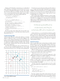
SVMs are quite difficult to understand, and they’re extremely difficult to implement. Take a look at the graph in Figure 3. The goal is to create a rule that distinguishes between the red data and the blue data. The graph shows a problem where the data has just two dimensions (number of predictor variables) only so that the problem can be visualized, but SVMs can work with data with three or more dimensions.
An SVM works by finding the widest possible lane that sepa- rates the two classes and then identifies the one or more points from each class that are closest to the edge of the separating lane.
To classify a new, previously unseen data point, all you have to do is see which side of the middle of the lane the new point falls. In Figure 3, the circled red point at (0.3, 0.65) and the circled blue points at (0.5, 0.75) and (0.65, 0.6) are called the support vectors. In my head, however, I think of them as “support points” because I usually think of vectors as lines.
There are three major challenges that must be solved to imple- ment a useable SVM. First, what do you do if the data isn’t linearly separable as it is in Figure 3? Second, just how do you find the support vectors, weights and biases values? Third, how do you deal with training data points that are anomalous and are on the wrong side of the boundary lane?
SVMs are quite difficult to understand, and they’re extremely difficult to implement.
As this article shows, you can deal with non-linearly separable data by using what’s called a kernel function. You can determine the support vectors, weights and biases using an algorithm called sequential minimal optimization (SMO). And you can deal with inconsistent training data using an idea known as complexity, which penalizes bad data.
Kernel Functions
There are many different types of kernel functions. Briefly, a kernel function takes two vectors and combines them in some way to produce a single scalar value. Although it’s not obvious, by using a kernel function, you can enable an SVM to handle data that’s not linearly separable. This is called “the kernel trick.”
Suppose you have a vector v1 = (3, 5, 2) and a second vector v2 = (4, 1, 0). A very simple kernel is called the linear kernel and it returns the sum of the products of the vector elements:
K(v1,v2)=(3*4)+(5*1)+(2*0)=17.0
Many kernel functions have an optional scaling factor, often
called gamma. For the previous example, if gamma is set to 0.5, then: K(v1,v2)=0.5*[(3*4)+(5*1)+(2*0)]=8.5
The demo program uses a polynomial kernel with degree = 2, gamma = 1.0 and constant = 0. In words, you compute the sum of products, then multiply by gamma, then add the constant, then raise to the degree. For example:
K(v1,v2)=[1.0*((3*4)+(5*1)+(2*0))+0]^2=(1*17+0)^2=289.0 The polynomial kernel is implemented by the demo program
like so:
public double PolyKernel(double[] v1, double[] v2) {
1.0 0.9 0.8 0.7 0.6 0.5 0.4 0.3 0.2 0.1 0.0
0.0 1.0 2.0 3.0
double sum = 0.0;
for (int i = 0; i < v1.Length; ++i)
sum += v1[i] * v2[i];
double z = this.gamma * sum + this.coef; return Math.Pow(z, this.degree);
Figure 3 Basic SVM Concepts 38 msdn magazine
The values of gamma, degree and constant (named coef to avoid a name clash with a language keyword) are class members and their values are supplied elsewhere. The demo program hard codes the
Machine Learning
4.0 5.0 6.0 7.0 8.0 9.0 1.0 x0
}
x1