Page 20 - MSDN Magazine, November 2018

Learning continues throughout the entire process. Essentially, this is the notion of delayed gratification, and it’s in the agent’s best inter- est not to be totally greedy so it leaves some room for exploration.
Testing the Epsilon Greedy Hypothesis
8 6 4
20
To test this hypothesis, add the code in Figure 2 to a new cell and execute it. This code creates the multi_armed_bandit function, which simulates a series of runs against a collection of slot machines. The function stores the observed odds of a jackpot pay- out. At each iteration, the agent will randomly play the slot machine with the best payout it has observed thus far, or arbitrarily try another machine. The argmax function returns the highest value in the numpy array. Here, that means the slot machine with the best odds of hitting a jackpot. The function’s parameters allow for control over the number of slot machines, the amount of iterations to run and the value of epsilon.
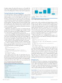
With the RL code in place, now it’s time to test the Epsilon Greedy algorithm. Enter the code from Figure 3 into an empty cell and execute it. The results show the chart from Figure 1 for easy refer- ence, followed by the odds that the RL code observed.
As you can see in Figure 4, the algorithm did an excellent job, not only of determining the slot machine with the most favorable odds, but also producing fairly accurate payout probabilities for the other four slot machines. The graphs line up rather well. The exception being the fifth slot machine, which has such low odds of a payout that it scored negatively in the agent’s observations.
Now, with the baseline established, it’s time to experiment some more. What would happen if epsilon were set to zero, meaning that the algorithm will never explore? Enter the following code in a new cell and execute it to run that experiment:
print("\n----------------------------------") print ("Learned Odds with epsilon of 0") print("----------------------------------") learned_payout_odds, reward =
multi_armed_bandit(number_of_slot_machines, iterations, 0) plt.bar(np.arange(len(learned_payout_odds)),learned_payout_odds) plt.show()
print (learned_payout_odds)
print ("Reward: ", sum(reward))
The resulting chart shows with one value higher than zero. One machine dominates the others, making it quite clear that the agent found one machine and stuck with it. However, run the code several times and you may notice that occasionally an inter- esting pattern develops. There will be one or more machines with
Figure 3 Code to Compare the Actual Slot Machine Odds with the Agent’s Observations
01234
[ 5.38709677 2.66666667 5.72222222 8.34395604 -1. ] Reward: 7899
Figure 4 Results with an Epsilon Value of .1
negative values, with one machine with a higher than zero value. In these cases, the agent lost on a given machine and then won on another machine. Once the agent discovers a winning machine, it will stick with that machine, as it will be the machine that the argmax function will choose. If epsilon is set to zero, the agent may still explore, but it will not be intentional. As such, the observed slot machine odds are nowhere near the actual odds. It is also worth noting that the “greedy” method produces a lower reward score than when epsilon was set to .1. Greed, at least abso- lute greed, would appear to be counterproductive.
What if epsilon were set to 1, making the agent explore every time and not exploit at all? Enter the following code into a new cell and execute it:
print("\n----------------------------------")
print ("Learned Odds with epsilon of 1") print("----------------------------------")
learned_payout_odds, reward = multi_armed_bandit(number_of_slot_machines, iterations, 1) plt.bar(np.arange(len(learned_payout_odds)),learned_payout_odds) plt.show()
print (learned_payout_odds) print ("Reward: ", sum(reward))
The results will show that the agent did an excellent job of observing odds similar to those of the true odds, and the chart lines up very closely with Figure 1. In fact, the results of setting epsilon to 1 look very similar to when the value was .1. Take note of the Reward value, however, and there is a stark difference. The reward value when epsilon was set to .1 will nearly always be higher than when it’s set to 1. When the agent is set to only explore, it will try a machine at random at every iteration. While it may be learning from observation, it is not acting on those observations.
Wrapping Up
RL remains one of the most exciting spaces in artificial intelligence. In this article, I explored the Epsilon Greedy algorithm with the classic “Multi-Armed Bandit” problem, specifically drilling into the explore-or-exploit dilemma that agents face. I encourage you to further explore the trade offs by experimenting with different values of epsilon and larger amount of slot machines. n
Frank La Vigne works at Microsoft as an AI Technology Solutions professional where he helps companies achieve more by getting the most out of their data with analytics and AI. He also co-hosts the DataDriven podcast. He blogs regularly at FranksWorld.com and you can watch him on his YouTube channel, “Frank’s World TV” (FranksWorld.TV).
Thanks to the following technical expert for reviewing this article: Andy Leonard
print ("Actual Odds") plt.bar(np.arange(len(JPs)),JPs) plt.show()
print (JPs) print("----------------------------------")
iterations = 1000
print("\n----------------------------------")
print ("Learned Odds with epsilon of .1") print("----------------------------------")
learned_payout_odds, reward = multi_armed_bandit(number_of_slot_machines, iterations, .1) plt.bar(np.arange(len(learned_payout_odds)),learned_payout_odds) plt.show()
print (learned_payout_odds)
print ("Reward: ", sum(reward))
14 msdn magazine
Artificially Intelligent