Page 58 - MSDN Magazine, July 2018

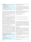
Figure 4 Training
After training, or during training, you’ll usually want to save the
model. In CNTK, saving would look like:
mdl_name = ".\\Models\\mnist_dnn.model" model.save(mdl_name)
This would save using the default CNTK v2 format. An alterna- tive is to use the Open Neural Network Exchange (ONNX) format. Notice that you’ll generally want to save the model object (with softmax activation) rather than the dnn object (no output activa- tion). From a different program, a saved model could be loaded
into memory along the lines of:
mdl_name = ".\\Models\\mnist_dnn.model"
model = C.ops.functions.Function.load(mdl_name)
After loading, the model can be used as if it had just been trained. The demo program doesn’t use the trained model to make a pre- diction. Prediction code could resemble this:
input_list = [0.55] * 784 # [0.55, 0.55, . . 0.55] input_vec = np.array(input_list, dtype=np.float32) pred_probs = model.eval(input_vec)
pred_digit = np.argmax(pred_probs) print(pred_digit)
Many neural network libraries use the term “epoch” to refer to one pass through all training items.
The input_list has a dummy input of 784 pixel values, each with value 0.55 (recall the model was trained on normalized data so you must feed in normalized data). The pixel values are copied into a NumPy array. The call to the eval function would return an array of 10 values that sum to 1.0 and can loosely be interpreted as probabilities. The argmax function returns the index (0 through 9) of the largest value, which is conveniently the same as the predicted digit. Neat!
Wrapping Up
Using a deep neural network used to be the most common approach for simple image classification. However, DNNs have at least two key limitations. First, DNNs don’t scale well to images that have a huge number of pixels. Second, DNNs don’t explicitly take into account the geometry of image pixels. For example, in an MNIST image, a pixel that’s directly below a second pixel is 28 positions away from first pixel in the input file.
Because of these limitations, and for other reasons, too, the use of a convolutional neural network (CNN) is now more common for image classification. That said, for simple image classifica- tion tasks, using a DNN is easier and often just as (or even more) effective than using a CNN. n
Dr. James mccaffrey works for Microsoft Research in Redmond, Wash. He has worked on several Microsoft products, including Internet Explorer and Bing. Dr. McCaffrey can be reached at jamccaff@microsoft.com.
Thanks to the following Microsoft technical experts who reviewed this article: Chris Lee, Ricky Loynd, Ken Tran
print("\nStarting training \n") for i in range(0, max_iter):
curr_batch = rdr.next_minibatch(batch_size, \ input_map=mnist_input_map)
trainer.train_minibatch(curr_batch) if i % int(max_iter/10) == 0:
mcee = trainer.previous_minibatch_loss_average macc = (1.0 - \
trainer.previous_minibatch_evaluation_average) \ * 100
print("batch %4d: mean loss = %0.4f, accuracy = \ %0.2f%% " % (i, mcee, macc))
If you examine the create_reader code in Figure 3, you’ll see that it specifies the tag names (“pixels” and “digit”) used in the data file. You can consider create_reader and the code to create a reader object as boilerplate code for DNN image classification problems. All you have to change is the tag names, and the name of the map- ping dictionary (mnist_input_map).
After everything is prepared, training is performed, as shown in Figure 4.
The demo program is designed so that each iteration processes one batch of training items. Many neural network libraries use the term “epoch” to refer to one pass through all training items. In this example, because there are 1,000 training items, and the batch size is set to 50, one epoch would be 20 iterations.
An alternative to training with a fixed number of iterations is to stop training when loss/error drops below some threshold. It’s important to display loss/error during training because training failure is the rule rather than the exception. Cross-entropy error is difficult to interpret directly, but you want to see values that tend to get smaller. Instead of displaying average classification error (“25 percent wrong”), the demo computes and prints the average classification accuracy (“75 percent correct”), which is a more natural metric in my opinion.
Evaluating and Using the Model
After an image classifier has been trained, you’ll usually want to evaluate the trained model on test data that has been held out. The demo computes classification accuracy as shown in Figure 5.
A new data reader is created. Notice that unlike the reader used for training, the new reader doesn’t traverse the data in random order, and that the number of sweeps is set to 1. The mnist_ input_map dictionary object is recreated. A common mistake is to try and use the original reader—but the rdr object has changed so you need to recreate the mapping. The test_minibatch function returns the average classification error for its mini-batch argument, which in this case is the entire 100-item test set.
Figure 5 Computing Classification Accuracy
rdr = create_reader(test_file, input_dim, output_dim, rnd_order=False, m_swps=1)
mnist_input_map = {
X : rdr.streams.x_src, Y : rdr.streams.y_src
}
num_test = 100
test_mb = rdr.next_minibatch(num_test,
input_map=mnist_input_map)
test_acc = (1.0 - trainer.test_minibatch(test_mb)) * 100 print("Model accuracy on the %d test items = %0.2f%%" \
% (num_test,test_acc)))
52 msdn magazine
Test Run