Page 22 - MSDN Magazine, July 2018

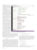
input values are (6,1, 3.1, 5.1, 1.1) and the output values are (0.0321, 0.6458, 0.3221). Figure 1 shows how the model was developed and trained. I used Visual Studio Code, but there are many alternatives.
This particular example involves predicting the species of an iris flower using input values that rep- resent sepal (a leaf-like structure) length and width and petal length and width. There are three possible species of flower: setosa, versicolor, virginica. The output values can be interpreted as probabilities (note that they sum to 1.0) so, because the second value, 0.6458, is larg- est, the model’s prediction is the second species, versicolor.
In Figure 2, each line connect- ing a pair of nodes represents a weight. A weight is just a numeric constant. If nodes are zero-base indexed, from top to bottom, the weight from input[0] to hidden[0] is 0.2680 and the weight from hidden[4] to output[0] is 0.9381.
Each hidden and output node has a small arrow pointing into the node. These are called biases. The bias for hidden[0] is 0.1164 and the bias for output[0] is -0.0466.
You can think of a neural network
as a complicated math function
because it just accepts numeric
input and produces numeric out-
put. An ML model on an IoT device
needs to know how to compute output. For the neural network in Figure 2, the first step is to compute the values of the hidden nodes. The value of each hidden node is the hyperbolic tangent (tanh) func- tion applied to the sum of the products of inputs and associated weights, plus the bias. For hidden[0] the calculation is:
hidden[0] = tanh((6.1 * 0.2680) + (3.1 * 0.3954) +
(5.1 * -0.5503) + (1.1 * -0.3220) + 0.1164)
= tanh(-0.1838) = -0.1817
Hidden nodes [1] through [4] are calculated similarly. The tanh function is called the hidden layer activation function. There are other activation functions that can be used, such as logistic sigmoid and rectified linear unit, which would give different hidden node values.
After the hidden node values have been computed, the next step is to compute preliminary output node values. A preliminary output node value is just the sum of products of hidden nodes and associ- ated hidden-to-output weights, plus the bias. In other words, the same calculation as used for hidden nodes, but without the activation function. For the preliminary value of output[0] the calculation is:
16 msdn magazine
Machine Learning
Figure 1 Creating and Training a Neural Network Model
o_pre[0] = (-0.1817 * 0.7552) + (-0.0824 * -0.7297) + (-0.1190 * -0.6733) + (-0.9287 * 0.9367) +
(-0.9081 * 0.9381) + (-0.0466) = -1.7654
The values for output nodes [1] and [2] are calculated in the same way. After the preliminary values of the output nodes have been com- puted, the final output node values can be converted to probabilities using the softmax activation function. The softmax function is best
explained by example. The calculations for the final output values are:
sum = exp(o_pre[0]) + exp(o_pre[1]) + exp(o_pre[2]) = 0.1711 + 3.4391 + 1.7153
= 5.3255
output[0]
output[1]
output[2]
= exp(o_pre[0]) / sum
= 0.1711 / 5.3255 = 0.0321
= exp(o_pre[1]) / sum
= 3.4391 / 5.3255 = 0.6458
= exp(o_pre[2]) / sum
= 1.7153 / 5.3255 = 0.3221
As with the hidden nodes, there are alternative output node activation functions, such as the identity function.