Page 24 - MSDN Magazine, March 2018

Input
b
x
w
Output
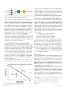
benign growths from the malignant ones. Logistic Regression is a simple linear model that takes input values (represented by the blue circles in Figure 4) of what I’m classifying and computes an output. Each of the input values has a different degree of weight on the output, depicted in Figure 4 as line thickness.
The next step is to minimize the error, or loss, using an optimi- zation technique. This notebook uses Stochastic Gradient Descent (SGD), a popular technique that usually begins by randomly ini- tializing the model parameters. In this case, the model parameters are the weights and biases. For each row in the data set, the SGD optimizer can calculate the error between the predicted value and the corresponding true value. The algorithm will then apply gradient descent to create new model parameters after each observation. SGD is explained in further detail inside the notebook and in a YouTube video by Siraj Raval (bit.ly/2B8lHEz).
The final step is to evaluate the predictive model’s performance against test data. There are essentially four outcomes for this binary classifier:
1. Correctly labeled the value as malignant. 2. Correctly labeled the value as benign.
3. Incorrectly labeled the value as malignant. 4. Incorrectly labeled the value as benign.
In this scenario, outcome No. 3 would be a false negative. The tumor is benign, but the algorithm flagged it incorrectly as malignant. This is also known as a Type II Error. Outcome No. 4 represents the reverse, a false positive. The tumor is malignant, but the algorithm marked it as benign, a Type I Error. More informa- tion about the Type I and II Errors, please refer to the Wikipedia article on erroneous outcomes of statistical tests at bit.ly/2DccUU8.
Using the plot in Figure 5, you can determine that the algorithm labeled three malignant tumors as benign, while not mislabeling any benign tumors as malignant.
Wrapping Up
The best way to quickly get started with exploring the various frameworks of data science, machine learning and artificial intel- ligence is through the DSVM image on Azure. It requires no installation or configuration, and it can be scaled up or down based on the problem to be solved. It’s a great way for people interested in machine learning to start experimenting right away. Best of all, the DSVM includes numerous Jupyter Notebook tutorials on the most popular machine learning frameworks.
In this article, I set up a DSVM and took the first steps into exploring the CNTK. By creating a binary classifier with logistic regression and Stochastic Gradient Descent, I trained an algorithm to determine whether or not a tumor was benign or malignant. While this model relied on only two dimensions and may not be ready for production, you did get an understanding of how this problem would be tackled in the real world. n
Frank La Vigne leads the Data & Analytics practice at Wintellect and co-hosts the DataDriven podcast. He blogs regularly at FranksWorld.com and you can watch him on his YouTube channel, “Frank’s World TV” (FranksWorld.TV).
Thanks to the following technical expert for reviewing this article: Andy Leonard
Artificially Intelligent
Figure 4 Diagram of Logistic Regression Algorithm
benign. This is a classification problem, specifically a binary clas- sification, as there are only two output classifications. To classify the type of growth in each patient, the hospital has provided the patient’s age and the size of his or her tumor. The working hypoth- esis is that that younger patients and patients with smaller tumors are less likely to have a malignant growth. Figure 3 shows how each patient in the data set is represented as a dot in the plot in the notebook. Red dots indicate malignant growths and blue dots indicate benign. The goal is to create a binary classifier to separate the malignant from the benign, similar to the scatter plot in the Out[3] cell in the notebook and duplicated in Figure 3.
The notebook includes a caution stating that the data set used here is merely a sample for educational purposes. A production classification system for determining the status of growths would involve more data points, features, test results and input from medical personnel to make the final diagnosis.
The Five Stages of a Machine Learning Project
Machine learning projects generally break down into five stages: Reading the data, shaping the data, creating a model, learning the model’s parameters and evaluating the model’s performance. Reading the data entails loading the data set into a structure. For Python, this generally means a Pandas DataFrame (bit.ly/2EPC8rI). DataFrames are essentially a tabular data structure consisting of rows and columns.
The second step is shaping the data from the input format into a format that the machine learning algorithm accepts. Often, this process is referred to as “data cleansing” or “data munging.” Very often this phase consumes the bulk of the time and effort in machine learning projects.
It’s not until the third stage that the actual machine learning work begins. In this notebook, I’ll create a model to separate the
Figure 5 Three Improperly Flagged Tumors 18 msdn magazine