Page 38 - MSDN Magazine, February 2018

normalization. In general, in non-demo scenarios you should normalize your predictor values.
Next, I wrote another utility program that took the 210-item data file in CNTK format, and then used the file to generate a 150-item training data file named seeds_train_data.txt (the first 50 of each variety) and a 60-item test file named seeds_test_data.txt (the last 20 of each variety).
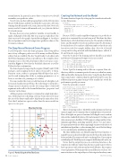
Because there are seven predictor variables, it’s not feasible to make a full graph of the data. But you can get a rough idea of the data’s structure by the graph of partial data in Figure 3. I used just the seed perimeter and seed compactness predictor values of the 60-item test dataset.
The Deep Neural Network Demo Program
I used Notepad to write the demo program. I like Notepad but most of my colleagues prefer one of the many excellent Python editors that are available. The free Visual Studio Code editor with the Python language add-in is especially nice. The complete demo program source code, with a few minor edits to save space, is pre- sented in Figure 4. Note that the backslash character is used by Python for line-continuation.
The demo begins by importing the required NumPy and CNTK packages, and assigning shortcut aliases of np and C to them. Function create_reader is a program-defined helper that can be used to read training data (if the is_training parameter is set to True) or test data (if is_training is set to False).
You can consider the create_reader function as boilerplate code for neural classification problems. The only things you’ll need to change in most situations are the two string values of the field arguments in the calls to the StreamDef function, “properties” and “varieties” in the demo.
All the program control logic is contained in a single main func- tion. All normal error checking code has been removed to keep the size of the demo small and to help keep the main ideas clear. Note that I indent two spaces rather than the more usual four spaces to save space.
Creating the Network and the Model
The main function begins by setting up the neural network archi- tecture dimensions:
def main():
print("Begin wheat seed classification demo") print("Using CNTK verson = " + str(C.__version__) ) input_dim = 7
hidden_dim = 4
output_dim = 3
...
Because CNTK is under rapid development, it‘s a good idea to print out or comment the version being used. The demo has three hidden layers, all of which have four nodes. The number of hidden layers, and the number of nodes in each layer, must be determined by trial and error. You can have a different number of nodes in each layer if you wish. For example, hidden_dim = [10, 8, 10, 12] would correspond to a deep network with four hidden layers, with 10, 8, 10, and 12 nodes respectively.
Next, the location of the training and test data files is specified and the network input and output vectors are created:
train_file = ".\\Data\\seeds_train_data.txt" test_file = ".\\Data\\seeds_test_data.txt"
# 1. create network and model
X = C.ops.input_variable(input_dim, np.float32) Y = C.ops.input_variable(output_dim, np.float32)
Notice I put the training and test files in a separate Data sub- directory, which is a common practice because you often have many different data files during model creation. Using the np.float32 data type is much more common than the np.float64 type because the additional precision gained using 64 bits usually isn't worth the performance penalty you incur.
Next, the network is created:
print("Creating a 7-(4-4-4)-3 NN for seed data ") with C.layers.default_options(init= \
C.initializer.normal(scale=0.1, seed=2)): h1 = C.layers.Dense(hidden_dim,
activation=C.ops.tanh, name='hidLayer1')(X)
h2 = C.layers.Dense(hidden_dim, activation=C.ops.tanh,
name='hidLayer2')(h1)
h3 = C.layers.Dense(hidden_dim, activation=C.ops.tanh,
name='hidLayer3')(h2)
oLayer = C.layers.Dense(output_dim, activation=None,
name='outLayer')(h3) nnet = oLayer
model = C.softmax(nnet)
There’s a lot going on here. The Python with statement is shortcut syntax to apply a set of common values to multiple layers of a network. Here, all weights are given a Gaussian (bell-shaped curve) random value with a standard deviation of 0.1 and a mean of 0. Setting a seed value ensures reproducibility. CNTK supports a large number of ini- tialization algorithms, including “uniform,” “glorot,” “he” and “xavier.” Deep neural networks are often surprisingly sensitive to the choice of initialization algorithm, so when training fails, one of the first things to try is an alternative initialization algorithm.
The three hidden layers are defined using the Dense function, so named because each node is fully connected to the nodes in the layers before and after. The syntax used can be confusing. Here, X acts as input to hidden layer h1. The h1 layer acts as input to hidden layer h2, and so on.
Notice that the output layer uses no activation function so the output nodes will have values that don’t necessarily sum to 1. If you have experience with other neural network libraries, this requires some explanation. With many other neural libraries you’d use soft- max activation on the output layer so that output value always sums
Machine Learning
1.00 0.98 0.96 0.94 0.92 0.90 0.88 0.86 0.84 0.82 0.80
10.00 11.00
Wheat Seed Test Data
Kama Rosa Canadian
12.00
13.00
14.00 Seed Perimeter
15.00
16.00
17.00
18.00
Figure 3 Partial Graph of the Test Data 34 msdn magazine
Seed Compactness