Page 20 - MSDN Magazine, December 15, 2017

Figure 2 Data Initialization and Model Training
Figure 3 A Typical Training Session Begins
data_frame = pd.read_csv("contoso_noisy.txt", names = ["level"])
input_count = 200 # How far to look back
output_count = 100 # How many steps forward to predict lstm_layer_output_dimensions = 128 # Size of LSTM output dropout_pct = 0.15 # Dropout density to avoid over-fitting
(training_inputs, training_targets, test_input) = dataframe_to_matrices(data_frame, input_count, output_count)
# How many input features? In this case, 1, but changes from model-to-model features = training_inputs.shape[2]
model = build_model(input_count, features, lstm_layer_output_dimensions,
output_count, dropout_pct)
# Train (Experimentally, ~0.12 seems to be an "elbow" --
lower ThresholdStop to gain accuracy by spending training time)
training_history = model.fit(training_inputs, training_targets, epochs=2500, batch_size=100, validation_split=0.15,
callbacks=[ThresholdStop(0.12)])
# Predict and output results, using input data held back from training predicted = model.predict(test_input)
>python Train.py
Using TensorFlow backend.
Train on 2295 samples, validate on 405 samples
Epoch 1/2500
2017-10-30 21:51:49.576493: W c:\\tf_jenkins\\home\\workspace\\release-win\\m\\ windows-gpu\\py\\35\\tensorflow\\core\\platform\\cpu_feature_guard.cc:45] The TensorFlow library wasn't compiled to use FMA instructions, but these are available on your machine and could speed up CPU computations. 2017-10-30 21:51:50.155264: I c:\\tf_jenkins\\home\\workspace\\release-win\\m\\ windows-gpu\\py\\35\\tensorflow\\core\\common_runtime\\gpu\\gpu_device.cc:940] Found device 0 with properties:
name: GeForce GTX 960M
major: 5 minor: 0 memoryClockRate (GHz) 1.0975
pciBusID 0000:01:00.0
Total memory: 2.00GiB
Free memory: 1.65GiB
2017-10-30 21:51:50.166001: I c:\\tf_jenkins\\home\\workspace\\release-win\\m\\ windows-gpu\\py\\35\\tensorflow\\core\\common_runtime\\gpu\\gpu_device.cc:1030] Creating TensorFlow device (/gpu:0) -> (device: 0, name: GeForce GTX 960M, pci bus id: 0000:01:00.0)
2295/2295 [======================] - 9s - loss: 4.4804 - val_loss: 2.8267 Epoch 2/2500
2295/2295 [======================] - 6s - loss: 3.0078 - val_loss: 2.8101 Epoch 3/2500
2295/2295 [======================] - 6s - loss: 2.8734 - val_loss: 2.6333 Epoch 4/2500
2295/2295 [======================] - 6s - loss: 2.5907 - val_loss: 2.2159 Epoch 5/2500
2295/2295 [======================] - 6s - loss: 1.8314 - val_loss: 1.1734 Epoch 6/2500
2295/2295 [======================] - 6s - loss: 0.9937 - val_loss: 0.7333 Epoch 7/2500
2295/2295 [======================] - 6s - loss: 0.7608 - val_loss: 0.6626 Epoch 8/2500
2295/2295 [======================] - 6s - loss: 0.6948 - val_loss: 0.6373 ...
The Long Short Term Memory (LSTM) cell looks back look- back_length samples at an input that has input_feature_count features. In this case, I have only one input feature: the input water levels at previous three-hour intervals. The output of the LSTM layer feeds into a densely interconnected layer that maps from an array of size lstm_layer_output_dimensions to an array of predic- tion_length that contains the model’s predictions of the water level at future intervals. Figure 1 shows a schematic of the architecture.
This is about as plain-vanilla a model as one could imagine for a time-series prediction problem. The LSTM cell is a kind of RNN.
The nitty-gritty of deep learning involves lots of parallel multiplication and sums over very large arrays of floating-point numbers.
Figure 2 shows how the model is built and trained. I use Pandas to read the training and validation data from the file contoso_noisy.txt and set the constants for a particular training experiment—in this case, looking back 200 steps, looking forward 100—with a 128-element hidden layer. The dropout_density sets a random percentage of input data to zero during training, which is immensely helpful for avoiding over-fitting (the problem of the model learning the specific training data and not generalizing to new situations). I convert the input data_frame to inputs and outputs for training and testing (the data-munging function data- frame_to_matrices isn’t shown, but is available in the source code distribution). I call the previously discussed build_model function and then call the model.fit function. This hours-long call adjusts the model’s internal values every 100 passes, and repeats either 2,500 times or once the error of the model drops below 12 percent of 1 foot, holding back 15 percent of the data for the validation step.
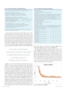
The first few epochs of a typical run are shown in Figure 3 and training and validation errors are shown in Figure 4.
Experienced ML developers might raise their eyebrows at the curves in Figure 4, which show the validation error (the test of the model against data held back from training) being less than that on the training data for quite a while; but the Loss curve includes that data held back by dropout, which artificially raises the error. The graph truncates the Y axis and so it doesn’t show the error for the first few dozen epochs. In general, it’s a pretty good curve, with no sign of overfitting, and pretty rapid convergence on an error around .15 percent of a foot, which is a little less than 2 inches. Pretty good for a noisy training set!
Figure 4 A Typical Training Run
16 msdn magazine
Machine Learning